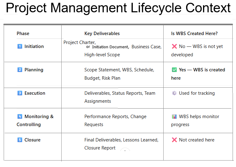
Top 10 Estimation Techniques in Project anagement

In project management, estimation is a critical process for predicting the time, cost, resources, and effort required to complete a project. Different estimation techniques are used depending on the project’s complexity, available data, and the stage of the project lifecycle. Below are the key estimation techniques used in project management:


1. Analogous Estimation (Top-Down Estimation)

  • Description: Uses historical data from similar past projects to estimate the current project.
  • When to Use: Early in the project when detailed information is limited.
  • Advantages:
    • Quick and easy to perform.
    • Requires minimal details.
  • Disadvantages:
    • Less accurate, as it relies on assumptions.
    • Not suitable for unique or complex projects.

2. Parametric Estimation

  • Description: Uses statistical relationships between historical data and project variables (e.g., cost per square foot, time per unit).
  • When to Use: When historical data is available and the project is well-defined.
  • Advantages:
    • More accurate than analogous estimation.
    • Scalable for large projects.
  • Disadvantages:
    • Requires reliable data and a clear understanding of variables.
    • May not account for unique project factors.

3. Bottom-Up Estimation

  • Description: Breaks the project into smaller tasks, estimates each task individually, and then aggregates the estimates.
  • When to Use: When detailed project information is available.
  • Advantages:
    • Highly accurate.
    • Provides a detailed understanding of the project.
  • Disadvantages:
    • Time-consuming.
    • Requires significant effort and expertise.

4. Three-Point Estimation

  • Description: Uses three estimates for each task:
    • Optimistic (O): Best-case scenario.
    • Pessimistic (P): Worst-case scenario.
    • Most Likely (M): Realistic scenario.
  • Formulas:
    • Triangular Distribution: Estimate=O+M+P3Estimate=3O+M+P
    • Beta Distribution (PERT): Estimate=O+4M+P6Estimate=6O+4M+P
  • When to Use: When there is uncertainty in task durations or costs.
  • Advantages:
    • Accounts for risks and uncertainties.
    • Provides a range of possible outcomes.
  • Disadvantages:
    • Requires more effort to calculate.
    • Relies on subjective judgment.

5. Expert Judgment

  • Description: Relies on the experience and intuition of experts to estimate project parameters.
  • When to Use: When historical data is unavailable or the project is unique.
  • Advantages:
    • Quick and flexible.
    • Useful for complex or innovative projects.
  • Disadvantages:
    • Subjective and prone to bias.
    • Accuracy depends on the expert’s experience.

6. Delphi Technique

  • Description: A structured method where experts provide estimates anonymously, and the results are aggregated and refined through multiple rounds of feedback.
  • When to Use: When consensus is needed among experts.
  • Advantages:
    • Reduces bias and groupthink.
    • Provides reliable estimates.
  • Disadvantages:
    • Time-consuming.
    • Requires coordination and facilitation.

7. Reserve Analysis

  • Description: Adds contingency reserves (time or cost) to the project estimate to account for uncertainties and risks.
  • When to Use: When the project has high uncertainty or risk.
  • Advantages:
    • Improves project resilience.
    • Accounts for unforeseen events.
  • Disadvantages:
    • Can lead to overestimation if not managed properly.

8. Comparative Estimation

  • Description: Compares the current project with similar past projects to estimate effort, cost, or duration.
  • When to Use: When historical data from comparable projects is available.
  • Advantages:
    • Simple and quick.
    • Useful for repetitive projects.
  • Disadvantages:
    • Less accurate for unique projects.
    • Relies on the availability of comparable data.

9. Function Point Analysis (FPA)

  • Description: Estimates the size and complexity of software projects based on the number of functions or features.
  • When to Use: For software development projects.
  • Advantages:
    • Standardized and objective.
    • Useful for measuring productivity.
  • Disadvantages:
    • Requires expertise in FPA.
    • Not suitable for non-software projects.

10. Monte Carlo Simulation

  • Description: Uses probability distributions and random sampling to simulate thousands of possible project outcomes.
  • When to Use: For complex projects with high uncertainty.
  • Advantages:
    • Provides a range of possible outcomes and probabilities.
    • Accounts for risks and uncertainties.
  • Disadvantages:
    • Requires specialized software and expertise.
    • Time-consuming to set up and run.

Choosing the Right Estimation Technique

  • Early Project Stages: Use analogous estimation or expert judgment when details are limited.
  • Detailed Planning: Use bottom-up estimation or parametric estimation when more information is available.
  • High Uncertainty: Use three-point estimationMonte Carlo simulation, or reserve analysis.
  • Software Projects: Use function point analysis or story points (in Agile).

By selecting the appropriate estimation technique(s), project managers can improve the accuracy of their estimates and set realistic expectations for stakeholders.

What is Project Scheduling & Explain Briefly

Project scheduling is a critical aspect of project management that involves planning, organizing, and managing tasks and resources to ensure the project is completed on time. Below is a step-by-step explanation of how to create and manage a project schedule:


Step 1: Define Project Scope and Objectives

  • Understand the project goals: Clearly define what the project aims to achieve.
  • Identify deliverables: List all the outputs or outcomes the project will produce.
  • Set boundaries: Determine what is included and excluded from the project scope.

Step 2: Break Down the Work (Work Breakdown Structure – WBS)

  • Decompose the project: Divide the project into smaller, manageable tasks or work packages.
  • Hierarchical structure: Organize tasks into levels (e.g., phases, deliverables, sub-tasks).
  • Ensure completeness: Make sure all tasks are accounted for to avoid missing critical work.

Step 3: Define Task Dependencies

  • Identify relationships: Determine the order in which tasks must be completed.
  • Types of dependencies:
    • Finish-to-Start (FS): Task B cannot start until Task A is finished.
    • Start-to-Start (SS): Task B cannot start until Task A starts.
    • Finish-to-Finish (FF): Task B cannot finish until Task A finishes.
    • Start-to-Finish (SF): Task B cannot finish until Task A starts (rare).
  • Use a network diagram: Visualize task dependencies to understand the flow of work.

Step 4: Estimate Task Durations

  • Gather input: Consult team members or experts to estimate how long each task will take.
  • Consider resources: Account for the availability of resources (e.g., people, equipment).
  • Use estimation techniques:
    • Expert judgment: Rely on experienced team members.
    • Analogous estimating: Use data from similar past projects.
    • Parametric estimating: Use statistical relationships (e.g., cost per unit).
    • Three-point estimating: Calculate optimistic, pessimistic, and most likely durations.

Step 5: Assign Resources

  • Identify resources: Determine the people, equipment, and materials needed for each task.
  • Allocate resources: Assign resources to tasks based on availability and skills.
  • Avoid over-allocation: Ensure resources are not overburdened by too many tasks.

Step 6: Develop the Schedule

  • Choose a scheduling tool: Use tools like Gantt charts, Microsoft Project, or software like Asana, Trello, or Jira.
  • Input tasks, durations, and dependencies: Populate the tool with the information gathered.
  • Set milestones: Identify key points in the project timeline (e.g., project phases, deliverables).
  • Calculate critical path: Identify the longest sequence of dependent tasks that determine the project duration.

Step 7: Review and Optimize the Schedule

  • Check for feasibility: Ensure the schedule is realistic and achievable.
  • Identify bottlenecks: Look for tasks that could delay the project.
  • Optimize resource allocation: Adjust resources to balance workloads.
  • Consider buffers: Add contingency time for high-risk tasks.

Step 8: Baseline the Schedule

  • Finalize the schedule: Once approved, set the schedule as the baseline.
  • Document assumptions: Record any assumptions made during scheduling.
  • Communicate the schedule: Share the baseline schedule with stakeholders and team members.

Step 9: Monitor and Control the Schedule

  • Track progress: Regularly compare actual progress to the baseline schedule.
  • Update the schedule: Adjust the schedule as needed to reflect changes or delays.
  • Manage changes: Use a change control process to handle scope or schedule changes.
  • Communicate updates: Keep stakeholders informed of any changes to the schedule.

Step 10: Close the Project

  • Review the schedule: Analyze how well the schedule was followed and identify lessons learned.
  • Document variances: Record any deviations from the baseline schedule.
  • Archive the schedule: Store the final schedule for future reference.

Key Tools and Techniques for Project Scheduling

  • Gantt Charts: Visual representation of tasks and timelines.
  • Critical Path Method (CPM): Identifies the longest path of dependent tasks.
  • Program Evaluation and Review Technique (PERT): Uses probabilistic time estimates.
  • Kanban Boards: Visual workflow management tool.
  • Resource Leveling: Balances resource allocation to avoid overloading.

Multidimensional Data Cube or Model, (Roll-up, Drill-Down Slice Dice) Operation

The Multidimensional data cube is a multi-dimensional array of data used for OLAP (Online Analytical Processing)

A Multidimensional data cube allows data to be viewed in multiple dimensions.

1. Roll-Up or Drill Up Operation

Roll-up is an aggregation operation that summarizes data by climbing up a concept hierarchy or by dimension reduction. It’s like zooming out to see a broader view.

Example: Sales data cube with dimensions: Location (City), Time (Month), and Product.

A roll-up operation might aggregate sales data from the city level to the country level.

Below Data Before Roll-Up:

  • City: Sales in New York, Los Angeles, Chicago
  • Month: January, February, March
  • Product: Laptops, Tablets, Phones

Below Data After Roll-Up:

  • Country: Sales in USA
  • Quarter: Q1
  • Product: Laptops, Tablets, Phones

2. Drill-Down Operation

Drill-down is the reverse of roll-up. It provides more detailed data by descending a concept hierarchy or adding dimensions. It’s like zooming in to see finer details.

Example: Using the same sales data cube, a drill-down operation might break down sales data from the country level to the city level.

Below Data Before Drill-Down:

  • Country: Sales in USA
  • Quarter: Q1
  • Product: Laptops, Tablets, Phones

Below Data After Drill-Down:

  • City: Sales in New York, Los Angeles, Chicago
  • Month: January, February, March
  • Product: Laptops, Tablets, Phones

3. Slice Operation

Slice selects a single dimension from the data cube, creating a sub-cube by fixing a value for one dimension.

Selection on one dimension of the given cube, resulting in a sub cube.

Example: If we want to analyze sales data for January only, we perform a slice operation on the Time dimension.

Below Data Before Slice:

  • City: Sales in New York, Los Angeles, Chicago
  • Month: January, February, March
  • Product: Laptops, Tablets, Phones

Below Data After Slice:

  • City: Sales in New York, Los Angeles, Chicago
  • Month: January
  • Product: Laptops, Tablets, Phones

4. Dice Operation

Dice selects two or more dimensions to create a sub-cube by fixing values for those dimensions.

Selection on two or more dimension of the given cube, resulting in a sub cube.

Example: If we want to analyze sales data for January and February in New York and Los Angeles, we perform a dice operation.

Below Data Before Dice:

  • City: Sales in New York, Los Angeles, Chicago
  • Month: January, February, March
  • Product: Laptops, Tablets, Phones

Below Data After Dice:

  • City: Sales in New York, Los Angeles
  • Month: January, February
  • Product: Laptops, Tablets, Phones

Multidimensional Data Model & Data Cubes with Example

A Multidimensional Data Model:: It is defined as a Data Model that allows data to be organized and viewed in multiple dimensions, such as time, item, branch, and location, enabling organizations to analyze relationships between different perspectives and entities efficiently.

A multidimensional data model views data in the form of a data cube, which allows data to be modeled and viewed in multiple dimensions. The key components are:

  • Dimensions: These are the perspectives or entities concerning which an organization keeps records. For example, time, item, and location.
  • Facts / Measures: These are the numerical measures or quantities. For example, sales amount.

Data Cube:: It is a multi-dimensional data structure. A data cube is organized by its dimensions (as Products, States, Date)

A data cube allows data to be viewed in multiple dimensions.

Example

A Retail store that wants to analyze its sales data. The dimensions could be:

  • Time: Year, Quarter, Month
  • Item: Product Category, Product Name
  • Location: City, Store

Dimensions:

  • Time: Q1, Q2, Q3, Q4
  • Item: Electronics, Clothing, Groceries
  • Location: New York, Los Angeles, Chicago

Conceptual Modeling of Data Warehouses & Its Schema as Star, Snowflake & Fact Constellation

Conceptual modeling is the high-level design phase of a data warehouse, focusing on how data is organized and represented for easy querying and reporting. It helps structure data in a way that supports analytical processing and business intelligence.

Conceptual Modeling defines high level design structure / schema of Data Warehouse, how data organized, reporting & querying etc.

Step [1] – Star schema is a most widely used schema design in data warehousing.

Star schema Features: It’s having central fact table that holds the primary data or measures, such as sales, revenue, or quantities. The fact table is connected to multiple dimension tables, each representing different attributes or characteristics related to the data in the fact table. The dimension tables are not directly connected to each other

Star Schema easy to understand & implement & best for reporting and OLAP (Online Analytical Processing)

Step [2] – Snowflake Schema is a extended part of Star Schema, where dimensions tables are normalized & connected with each others.

Snowflake Schema is more complex schema where dimension tables are normalized into multiple related tables.

Snowflake Features: It’s having central fact table that holds the primary data or measures, such as sales, revenue, or quantities. The fact table is connected to multiple dimension tables, each representing different attributes or characteristics related to the data in the fact table. The dimension tables are directly connected to each other

Star Schema easy to understand & implement & best for reporting and OLAP (Online Analytical Processing)

How Data Warehouse Support ETL (Extract, Transform, and Load)

Extract, transform, and load (ETL) is the process of combining data from multiple sources into a large, central repository called a data warehouse. ETL uses a set of business rules to clean and organize raw data and prepare it for storage, Business Intelligence, Data Analytics, and Machine Learning (ML).

Collect raw data from various sources (databases, APIs, flat files, etc.).

Step [1]- Extract Data: ETL process is used to extract data from various sources such as transactional systems, spreadsheets, and flat files. This step involves reading data from the source systems and storing it in a staging area.

Clean, filter, and format raw data to match the data warehouse schema.

Step [2] – Transform Data: The extracted data is transformed into a format that is suitable for loading into the data warehouse. This may involve cleaning and validating the data, converting data types, combining data from multiple sources, and creating new data fields.

Store transformed data into the data warehouse for reporting and analysis.

Step [3] – Load Data: Once Data transformed, it is loaded into the data warehouse. This step included creating the physical data structures and loading the data into the warehouse.

ETL Working Flow in Data Warehouse

Differentiate among Data Swap, Data Puddles, Data warehouse & Data Lake with Examples.

1. Data Swap (Data Mart)

A Temporary storage location where data is exchanged or transferred between two systems, It typically handles small transactional data in a structured format.

  • Definition: A small, focused subset of a data warehouse designed for a specific department or team.
  • Scope: Limited to a single business unit (e.g., Sales, Marketing).
  • Purpose: Quick access to relevant data for specific needs.
  • Structure: Highly structured and pre-processed.
  • Example:
    • A sales data mart containing monthly sales, customer data, and product performance for the sales department.
    • I a E-commerce, when a customer makes a payment , the payment gateway system exchanges transaction details with the Order Mgt System.

2. Data Puddles

Small, isolated collections or data typically focused on a specific department or project. These are often uncoordinated & may no follow a consistent schema.

  • Definition: A small-scale, isolated data repository created by individual teams for short-term use.
  • Scope: Project or Department specific or team-specific with minimal governance.
  • Purpose: Temporary storage for ad-hoc analysis or experiments.
  • Structure: Semi-structured or unstructured, often created for quick insights.
  • Example:
    • A marketing team’s Excel sheets and Google Drive files collecting social media metrics for a campaign.
    • It serves marketing specific needs but is not accessible across other departments.

3. Data Warehouse

A centralized repository of structured data that is cleaned, organized & optimized for querying & reporting.
Data Warehouses support Business Intelligence(BI) & analytics by integrating data from multiple sources.

  • Definition: A centralized, structured repository that stores processed and organized data from multiple sources.
  • Scope: Enterprise-wide, integrating data from across the organization.
  • Purpose: Supports business intelligence (BI), reporting, and analysis.
  • Structure: Highly structured with defined schemas (star/snowflake schemas).
  • Example:
    • Amazon Redshift or Google BigQuery storing customer transactions, inventory, and supply chain data for reporting and forecasting.
    • An otg

4. Data Lake

A scalable repository that stores vast amounts of data as

Structured Data Format, Unstructured Data Format, Semi Structured Data Format.

It is used for advanced analytics, machine learning & big data

  • Definition: A vast, unstructured repository that stores raw data from various sources in its native format.
  • Scope: Enterprise-wide with the ability to store massive datasets.
  • Purpose: Enables advanced analytics, machine learning (ML), and data discovery.
  • Structure: Unstructured or semi-structured; no predefined schema.
  • Example:
    • AWS S3 or Azure Data Lake storing IoT sensor data, social media feeds, and raw logs for future analysis.
    • An organization uses data warehouse (Snowflake or Amazon redshift) to coordinate sales, customer & financial data, It allows analysts to create dashboards & generate reports for long term business strategy.

Key Differences

AspectData Swap (Mart)Data PuddleData WarehouseData Lake
ScopeDepartment-specificProject or team-specificOrganization-wideOrganization-wide
Data StructureStructuredSemi-structured/unstructuredStructuredUnstructured/semi-structured
Data VolumeSmall to mediumSmallLargeVery large
PurposeSpecific business unit reportingTemporary/quick analysisReporting & BIAdvanced analytics & big data
Storage FormatPre-processedRawPre-processedRaw
ProcessingMinimalMinimalExtensive ETLELT (Extract, Load, Transform later)
ExampleSales Mart for KPIsExcel files for project insightsEnterprise-wide BI reportsIoT sensor and video data repository

Explain Activity Diagram, Network Diagram, Forward Pass, and Backward Pass

Step-1: Activity Diagram:

  • A flowchart that visually represents the sequence of activities and decisions in a process or project. It shows the flow from one activity to another but lacks time or resource detail.
  • Used primarily in UML (Unified Modeling Language) for software modeling.

Step-2: Network Diagram:

  • A graphical representation of a project’s activities and their dependencies. It shows the order and sequence of tasks using nodes (activities) and arrows (dependencies).
  • Two types:
    • AOA (Activity on Arrow) – Arrows represent activities.
    • AON (Activity on Node) – Nodes represent activities (most common).

Step-3: Forward Pass:

  • Calculates the earliest start (ES) and earliest finish (EF) times for each activity, beginning at the project start.
  • Formula:

Step-4: Backward Pass:

  • Determines the latest start (LS) and latest finish (LF) times by moving backward from the project’s end.
  • Formula:

Differences Between Activity Diagrams, Network Diagrams, and Gantt Charts

AspectActivity DiagramNetwork DiagramGantt Chart
PurposeModels workflows/processesMaps activity dependenciesTracks task schedules over time
VisualizationFlowchart of activitiesNodes (tasks) and arrows (dependencies)Bars showing task duration and overlap
Time RepresentationNo time elementShows project timeline and dependenciesDirectly shows duration, progress, and deadlines
FocusWorkflow, software modelingCritical path and task dependenciesSchedule tracking and resource allocation
Use CaseSoftware and system modelingProject planning and schedulingProject management and tracking progress

Step-5: Calculating the Critical Path

  • Critical Path:
    • The longest path through the network diagram. It shows the sequence of tasks that determine the shortest project duration. Any delay in the critical path delays the project.

Steps to Calculate Critical Path:

  1. List all project activities and durations.
  2. Identify dependencies (predecessors).
  3. Draw the network diagram.
  4. Perform forward and backward passes.
  5. Calculate slack for each activity.
  6. The path with zero slack is the critical path.

Step-6: Calculating Slack (Float)

  • Slack:
    • The amount of time an activity can be delayed without delaying the project.
    • Formula:
    • Zero Slack indicates the activity is on the critical path.

How To Create Pivot Table & Pivot Chart

The following things need to be followed

Step [1] – Before Pivot Table Ensure Your Data Correct Format

Ensure your data is structured correctly.

  • Format: Use a table or list format with clear headers in the first row.
  • No Blank Rows/Columns: Ensure there are no empty rows or columns within the dataset.
  • Consistent Data: Data should be consistent (e.g., dates in one column, numbers in another).

Step [2] –

[2.1]Select the Data: Highlight the entire dataset (including headers).

[2.2] – Go to “Insert” Tab: Click on the “Insert” tab in Excel.

[2.3] – Choose Pivot Table:

  • Click on “Pivot Table” in the Tables group.

[2.4]- Select Pivot Table Location:

  • New Worksheet: Places the Pivot Table in a new sheet. or
  • Existing Worksheet: Allows you to specify the location.

Note:: For best result always try to select New Worksheet

[2.5] – Click “OK.”

Step [3] – Build the Pivot Table

Filters (Optional): Add a field to the Filters area to filter data dynamically.

A blank Pivot Table field list appears.

Drag and Drop Fields:

Rows: Drag a categorical field (e.g., Physical store, Country Name) into the “Rows” area.

Values: Drag a numerical field (e.g., List Price, Actual Price) into the “Values” area.

Columns (Optional): Drag another field (e.g., Date) to see data across columns.

Step [4] – Physical Store in Rows & List Price in Values, by default List Price display sum of list price corresponding to physical store.

[4.1] – Grand Total = Sum of all Physical Store List Price

[4.2] – Right Click any of (rows) Numeric value of (Sum of List Price)–>display

  • Sort
  • Summarize Values By
  • Show Values At

[4.3] – Summarize Values By

[a] – If Select Summarize Values By –> Count , result as

[b] – If Select Summarize Values By –> Average , result as

Once Select — Summarize Values By –> Average

[c] – If Select Summarize Values By –> Max , result as

Once Select — Summarize Values By –> Max

[d] – If Select Summarize Values By –> Min , result as

Once Select — Summarize Values By –> Min

[4.4] – Show Values As

–Once Select — Show Values As –> % of Grand Total

[4.5] – Sort->Smallest To Largest or Sort->Largest To Smallest

[a] Sort->Smallest To Largest result

[b] Sort->Largest To Smallest result

What are Herzberg Two-Factor Theory or Motivation-Hygiene Theory

Herzberg’s Two-Factor Theory:: It is also known as Motivation-Hygiene Theory::

Herzberg’s Two-Factor Theory or Motivation-Hygiene Theory is a foundational concept in understanding how to manage and motivate teams effectively. It focuses on two types of factors that influence job satisfaction and performance: motivators and hygiene factors.

Core Concepts of Herzberg’s Theory

1. Hygiene Factors (Extrinsic Factors)

  • These are basic workplace conditions and factors that prevent dissatisfaction but do not necessarily motivate employees to perform better.
  • Examples:
    • Salary and benefits
    • Job security
    • Work environment
    • Company policies
    • Relationships with colleagues and supervisors
  • If these factors are absent or inadequate, they lead to dissatisfaction. However, improving these factors alone won’t significantly increase motivation or satisfaction.

2. Motivators (Intrinsic Factors)

  • These factors are related to the nature of the work itself and are key to driving satisfaction and motivation.
  • Examples:
    • Achievement
    • Recognition
    • Responsibility
    • Personal growth and development
    • Meaningful work
  • The presence of motivators enhances satisfaction and inspires higher levels of performance.

Application of Herzberg’s Theory in Managing Teams

  1. Ensure Hygiene Factors Are in Place
    • Address and resolve complaints about work conditions, such as poor pay, unsafe environments, or outdated policies.
    • Maintain open communication channels to identify and mitigate dissatisfaction early.
  2. Focus on Motivators for Engagement
    • Empower team members by giving them autonomy and responsibilities that align with their strengths and career goals.
    • Provide opportunities for growth through training, upskilling, and challenging projects.
    • Recognize and celebrate achievements to boost morale and motivate individuals.
  3. Tailor Management Strategies
    • Understand individual team members’ motivators. For example, one person might value public recognition, while another may prioritize professional development.
    • Align tasks and responsibilities with what employees find meaningful and fulfilling.
  4. Create a Balance
    • While hygiene factors are essential to create a foundation of satisfaction, motivators are what drive sustained performance and engagement.
    • Combine practical improvements (e.g., competitive salaries and benefits) with intrinsic rewards (e.g., opportunities for innovation).
  5. Encourage Feedback and Adaptation
    • Regularly seek input from the team about what works and what doesn’t. This helps refine both hygiene and motivator strategies to meet the team’s evolving needs.

Practical Example

Imagine a project team working under tight deadlines:

  • Hygiene focus: Ensure the team has access to necessary resources, a comfortable work environment, and clear communication about goals.
  • Motivator focus: Recognize milestones achieved during the project, offer opportunities for leadership within the team, and highlight how their work contributes to the organization’s success.

By integrating Herzberg’s theory into team management, leaders can reduce dissatisfaction while fostering a motivated and high-performing team.