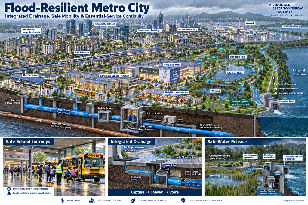
Rain-Ready City” and “Sponge Metropolis” through conceptual 3D architectural visualizations
Heavy rainfall tests the connections that make a city work. A flooded road can interrupt school transport. A submerged electrical installation can disable a pumping station. A waterlogged station entrance can make an otherwise operational metro line inaccessible.
A flood-resilient city plans for these interdependencies. Its buildings, streets, transport networks, public spaces, utilities, and emergency procedures work together to reduce damage and support essential services.
The two accompanying 3D concepts—the Rain-Ready City and the Sponge Metropolis—explore this approach. They illustrate possible planning principles, rather than construction-ready designs or guarantees of uninterrupted operation.
The practical ambition is clear: protect people, maintain essential services where conditions allow, and recover quickly when extreme rainfall exceeds the city’s capacity.
Two architectural visions with a shared purpose
The Rain-Ready City emphasizes connected canals, protected urban districts, elevated transport, and visible underground drainage. Water has designated routes through and around the city.
The Sponge Metropolis emphasizes distributed storage: green roofs, planted streets, rain gardens, floodable parks, and terraced basins. Its public landscape helps manage rainfall close to where it lands.
These approaches can complement one another. Green infrastructure captures and manages runoff, while conventional infrastructure provides additional conveyance and storage. The EPA describes green infrastructure as using vegetation, soils, permeable surfaces, and related measures to reduce and treat stormwater. EPA: Green Infrastructure
| Planning feature | Rain-Ready City concept | Sponge Metropolis concept |
|---|---|---|
| Main visual idea | Connected waterways and protected districts | Green neighborhoods and distributed water storage |
| Transport arrangement | Elevated routes and sheltered interchanges | Connected transit integrated with planted public spaces |
| Water-management emphasis | Collection, conveyance, storage, and controlled discharge | Capture, infiltration where suitable, storage, and reuse |
| Public-space role | Canal corridors and designated overflow areas | Rain gardens, wetlands, and floodable parks |
| Shared objective | Safer mobility and essential-service continuity | Safer mobility and essential-service continuity |
Start with the landscape before designing the skyline
A practical masterplan would begin with the catchment—the entire area contributing water to the city.
Planners would need to understand ground levels, natural drainage routes, historic flooding, soil conditions, groundwater, river levels, and downstream constraints. The same rainfall can produce very different consequences in a steep inland city, a low-lying coastal city, or a settlement beside a river.
Building elevations, transport routes, storage areas, and outlet locations should follow that assessment. Raising one district without considering surrounding areas could redirect water toward neighboring communities.
The World Bank’s integrated urban flood-risk approach combines physical infrastructure with planning, preparedness, and institutional coordination. This supports treating flood resilience as a citywide responsibility. World Bank: Cities and Flooding
Give rainwater a complete, connected journey
In both concepts, every neighborhood needs a defined route for runoff. A drain outside a building achieves little if the connecting network is blocked, undersized, or unable to discharge.
The proposed water journey has five stages:
- Capture: Roof gutters, street inlets, rain gardens, and permeable surfaces intercept rainfall.
- Convey: Local drains, planted channels, and trunk pipes move excess water toward storage.
- Store: Tanks, detention basins, and designated floodable spaces temporarily hold runoff.
- Treat and reuse: Suitable treatment supports selected uses such as irrigation or toilet flushing.
- Release: Controlled outlets discharge water when receiving conditions allow.
Not every location can absorb water effectively. Infiltration requires suitable soil, groundwater conditions, and contamination assessment. Where infiltration is unsuitable, planted systems can incorporate liners, underdrains, or controlled storage.
Stormwater and sewage are shown as separate networks in the concepts. Runoff still needs appropriate pollution management; keeping it separate from sewage does not automatically make it clean.
Storage capacity matters as much as drainage capacity
Moving water rapidly out of one neighborhood can increase pressure elsewhere. Temporary storage creates time between rainfall entering the system and water leaving the city.
The proposed basins would have defined operating levels and reserved capacity for storms. A visually attractive lake that is already full may provide little additional storage.
Likewise, the terraced ponds in the Sponge Metropolis image are conceptual representations. Their actual levels, connections, slopes, embankments, and overflow structures would require hydraulic and geotechnical design.
An external reservoir is also a finite receiving system. It cannot be assumed to accept unlimited discharge, particularly when the wider region is experiencing the same storm.
Plan for an outlet that cannot discharge
A critical operating scenario occurs when a receiving river or reservoir rises high enough to restrict drainage.
The concept therefore includes backflow protection, temporary storage, and pumping where justified. A closed backflow gate can prevent incoming water, but it also restricts outgoing gravity flow. The city must have somewhere to hold the water accumulating behind it.
Pumps would require protected electrical equipment, backup power, maintenance access, and operating procedures. Their discharge rates must remain compatible with downstream conditions.
For events exceeding normal capacity, designated surface overflow corridors would direct water away from occupied buildings and critical facilities. These areas would need access restrictions when activated.
Design each urban zone around its essential function
Flood protection should preserve access as well as buildings.
| Urban zone | Proposed infrastructure | Intended practical benefit |
|---|---|---|
| Residential neighborhoods | Elevated entrances, accessible ramps, local drainage, and rainwater storage | Reduce water entry and support safer access |
| Corporate offices | Protected utility rooms, backup systems, and alternative access | Support critical business operations |
| Government buildings | Protected communications, records, and emergency coordination facilities | Maintain public-service capability |
| Parking facilities | Raised parking, monitored entrances, and managed closure procedures | Reduce exposure of vehicles and users |
| Rail and metro | Protected entrances, track drainage, and accessible station connections | Support service where operating conditions permit |
| Airport | Airfield drainage, protected terminal access, and coordinated operating procedures | Reduce infrastructure-related disruption |
| Bus terminals | Sheltered boarding, drained pedestrian areas, and alternative routes | Support safer passenger transfers |
| Schools | Covered boarding, supervised access, shelter, and family communication | Protect children during changing conditions |
| Shopping malls | Protected access, loading arrangements, and critical equipment | Support safe commercial activity |
| Neighborhood markets | Covered walkways, accessible drainage, and waste collection | Support local trade and reduce drain blockage |
Elevated rail alone cannot ensure transport continuity: passengers still need safe routes to stations. Airport drainage likewise cannot eliminate restrictions caused by low visibility, lightning, wind, or other operational hazards.
Make school journeys a specific operating plan
School transport deserves particular attention because weather conditions may change between morning pickup and afternoon dismissal.
In this concept, a school journey would involve monitored routes, sheltered boarding, supervised pedestrian movement, and clear communication among the school, transport operator, drivers, and families.
Alternative routes would be assessed in advance. Schools would also need arrangements for delayed collection and supervised shelter.
If conditions become unsafe, transport would be suspended. Children should never be sent through floodwater simply to preserve a timetable. Successful continuity planning includes knowing when to stop an activity safely.
Use public landscapes as working infrastructure
The Sponge Metropolis places water-management functions within everyday spaces.
Rain gardens can receive runoff from nearby surfaces. Green roofs can retain part of the rainfall reaching buildings. Permeable paving can help manage runoff where ground conditions and maintenance arrangements support it. Wetlands and planted basins can provide water-management and ecological benefits. EPA: Types of Green Infrastructure
Floodable parks would require clear operating rules. They could serve recreation during suitable conditions and temporarily store water during storms, with public access closed when necessary.
These spaces would need inspection and cleanup before reopening. Their performance depends on maintenance and available capacity.
Connect monitoring to accountable decisions
Rain gauges, water-level sensors, pump-status monitoring, and road-condition reports could support a shared operational picture.
For these concepts, a city control team might use that information to inspect a rising basin, dispatch crews to a blocked inlet, close an underpass, reroute buses, or warn a school transport operator.
Each alert needs a named owner and an agreed response. Manual checks and backup communication would remain necessary when sensors, power, or connectivity fail.
Build maintenance into the investment
Infrastructure performance depends on what happens after construction.
The proposed operating program would include drain cleaning, debris-screen inspection, sediment removal, pump testing, backup-power checks, vegetation management, and inspection of gates and outlets.
Responsibility should be explicit across municipal agencies, transport operators, property owners, schools, and utility providers. Construction budgets should be accompanied by realistic funding for operation, inspection, and replacement.
Turn the vision into a phased project
An existing city could apply these ideas incrementally:
- Map flood pathways, service dependencies, and vulnerable populations.
- Address blocked drainage, dangerous crossings, and exposed essential equipment.
- Pilot improvements in a school district, market area, or transport interchange.
- Develop connected storage, drainage, and controlled outlet capacity.
- Expand successful measures using observed performance and updated modeling.
Progress could be measured through waterlogging duration, households affected, essential-service downtime, safe-route availability, maintenance completion, and recovery time. Targets would be set against local conditions and a defined baseline.
The strongest outcome would be a city where infrastructure decisions are judged by how well they protect everyday life: a child waiting safely at school, an ambulance retaining access, a household avoiding repeated water entry, and a public transport network recovering promptly after severe weather.
Image disclosure: The accompanying images are AI-generated conceptual architectural visualizations. They are not approved engineering designs. Implementation requires site-specific studies, qualified professional design, and relevant approvals.